Short answer
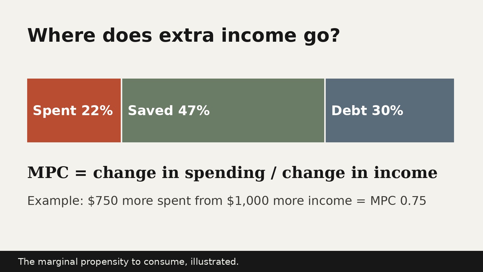
- The marginal propensity to consume, usually shortened to MPC, is the share of an extra dollar of income that a household spends on consumption rather than saving it. If income rises by $1,000 and spending rises by $750, the MPC is 0.75, or 75 percent. It is calculated as the change in consumption divided by the change in income. MPC matters because it links a change in income to a change in total spending, and through repeated rounds of spending it helps determine the size of the spending multiplier. This article is an economics explainer only. It is not personal financial advice, and it does not recommend any product, purchase, or financial decision.
What the marginal propensity to consume means
In economics, consumption means spending by households on goods and services: food, housing services, transport, clothing, health care, entertainment, and similar items. Income, in this context, usually means disposable income, which is income left after taxes and after adding transfers such as government benefits, depending on the exact definition being used. The U.S. Bureau of Economic Analysis defines disposable personal income as the income available to persons for spending or saving, equal to personal income less personal current taxes.
The word marginal is doing important work in the term. Marginal does not mean small or unimportant. It means “on the margin,” which is economist language for the next unit, the additional amount, or the change. MPC therefore does not ask what share of total income a household spends. It asks a narrower question: when income changes by some amount, how much of that change goes to consumption?
That distinction matters. A household might spend 90 percent of its total income on essentials and still have a low MPC, if it saves almost all of any pay rise. Another household might spend only 60 percent of its total income, yet spend most of a one off bonus. MPC describes the response to a change, not the overall spending pattern.
MPC is a central idea in Keynesian economics, the school of thought associated with John Maynard Keynes, which gives a large role to total spending, or aggregate demand, in determining economic activity in the short run. In that framework, a rise in income leads to a rise in spending, which becomes income for someone else, which leads to further spending, and so on. MPC measures the strength of each step in that chain. A higher MPC means more of each extra dollar is passed on as spending. A lower MPC means more leaks out of the spending chain into saving, at least in the simple version of the model. It is not a fixed law of nature, and it is not the same for every household, every type of income change, or every time period.
The MPC formula
The standard formula is simple:
MPC = change in consumption divided by change in disposable income
In symbols, this is often written as:
MPC = ΔC / ΔY
Here, ΔC is the change in consumption and ΔY is the change in disposable income. The Greek letter delta, Δ, simply means “change in.” Some textbooks write ΔYd for the change in disposable income, to make clear that taxes have already been taken out. The logic is identical.
Three points prevent common errors. First, both changes must refer to the same period and the same household or group. Second, the income change should be disposable income where possible, not gross pay: if a $1,000 pay rise leads to $200 in extra tax, disposable income rises by only $800. Third, consumption means spending on goods and services. In textbook models, debt repayment is often grouped with saving, because it increases net wealth rather than buying a current good or service, while survey research may treat it as a separate use of money. When you read an MPC estimate, check how the study treated debt repayment, because that choice changes the number.
To calculate MPC, find the change in disposable income, find the change in consumption over the same period, divide the second by the first, and read the result as a share. An MPC of 0.75 means 75 cents of each extra dollar is spent on consumption. An MPC of 0.20 means 20 cents of each extra dollar is spent.
A negative MPC is possible in principle if spending falls when income rises, but that is unusual and would usually signal that something else changed at the same time, such as a decision to pay down a large debt. An MPC above 1 is also possible in practice if a household borrows or draws on savings to spend more than the income rise itself. Textbook models often assume MPC lies between 0 and 1, but that is a modeling simplification, not a physical limit.
Worked examples
Example 1: A pay rise
Suppose a household receives a pay rise that increases disposable income by $1,000 per month. Its spending on goods and services rises by $750 per month, and it saves the remaining $250.
MPC = 750 / 1,000 = 0.75
The household spends 75 percent of the extra income and saves 25 percent.
Example 2: A one off payment
Suppose a household receives a one off payment of $500. It spends $200 on groceries, transport, and a household repair, saves $200, and uses $100 to pay down a credit card balance.
If debt repayment is grouped with saving, as in the simple textbook split, then consumption is $200 and the MPC is 200 / 500 = 0.40. If debt repayment is counted separately, the three way split is 40 percent spent, 40 percent saved, and 20 percent used to pay down debt. The MPC is still 0.40, because MPC counts only spending on goods and services. A study that lumps debt repayment together with spending would report a higher MPC than a study that separates them, even for identical behavior.
Example 3: Comparing two households
Household A receives an extra $2,000 and spends $1,800 of it. Its MPC is 1,800 / 2,000 = 0.90. Household B receives an extra $2,000 and spends $600 of it. Its MPC is 600 / 2,000 = 0.30. The equally weighted average across the two households is (0.90 + 0.30) / 2 = 0.60, but that average hides a large difference in behavior. If the income goes mainly to households like A, total spending rises much more than if it goes mainly to households like B. This variation across households, called heterogeneity, is one of the most important findings in modern MPC research.
Example 4: A fall in income
The same formula applies to falls. Suppose disposable income falls by $800 and consumption falls by $400, because the household cuts some discretionary spending but protects essentials and draws on savings for the rest. MPC = (negative 400) / (negative 800) = 0.50. In practice, spending often falls by less than income in the short run, because households try to smooth consumption by using savings or credit. Over a longer period, if the income fall persists, spending usually adjusts further.
MPC and average propensity to consume
MPC is often confused with the average propensity to consume, or APC. The two answer different questions. APC = total consumption divided by total income. It describes the overall spending share. MPC = change in consumption divided by change in income. It describes the spending response to a change.
| Income | Consumption | APC | MPC for the change | |
|---|---|---|---|---|
| Before | $4,000 | $3,600 | 0.90 | Not applicable |
| After | $5,000 | $4,350 | 0.87 | 0.75 |
Total income rose by $1,000 and total consumption rose by $750, so MPC is 750 / 1,000 = 0.75. The APC fell slightly, from 0.90 to 0.87, even though spending rose in absolute terms, because income grew faster than spending. A falling APC alongside a positive MPC is normal and is not a contradiction. For questions about the effect of a new payment, tax change, or pay rise, MPC is the relevant concept, because the question is about a change.
Marginal propensity to save
The marginal propensity to save, or MPS, is the share of an extra dollar of income that is saved rather than spent on consumption: MPS = change in saving divided by change in disposable income. In the simple two way split, where every extra dollar is either spent on consumption or saved, the two shares must add to 1:
MPC + MPS = 1
So if MPC is 0.75, MPS is 0.25. If MPC is 0.20, MPS is 0.80. This identity is arithmetic, not a discovery: it follows from the definition that the extra dollar is divided between the two uses.
In real life, the split is often more complicated, because extra income can also go to debt repayment, tax payments, or transfers to others. If debt repayment is counted separately, the identity becomes: share spent plus share saved plus share used to pay down debt equals 1. In that three way split, MPC plus MPS alone does not equal 1. For textbook multiplier calculations, the simple two way split is usually assumed, so MPS equals 1 minus MPC. When reading real world estimates, always check which split the study used before applying the identity.
The spending multiplier
The multiplier is the reason MPC matters beyond individual household budgets. When one household spends extra income, that spending becomes income for shopkeepers, workers, suppliers, and service providers. Those recipients then spend part of their new income, creating further income for others, and so on. The total increase in spending and income can therefore exceed the initial injection.
In the simplest textbook model, with no taxes, no imports, and no other leakages, the spending multiplier, often written as k, is:
k = 1 / (1 minus MPC) = 1 / MPS
The logic is a geometric series. Each round of spending is MPC times the previous round, so the total is 1 plus MPC plus MPC squared plus MPC cubed, continuing indefinitely, which sums to 1 / (1 minus MPC) when MPC is between 0 and 1.
Worked example with MPC = 0.80 and an initial injection of $1,000: round 1 spends $1,000, round 2 spends $800, round 3 spends $640, round 4 spends $512, round 5 spends $409.60, and so on. The running total after round 3 is $2,440, after round 4 is $2,952, and after all rounds it converges to $5,000, which matches the formula: k = 1 / (1 minus 0.80) = 1 / 0.20 = 5, and 5 times $1,000 = $5,000.
| MPC | MPS (simple split) | Multiplier k = 1 / MPS |
|---|---|---|
| 0.90 | 0.10 | 10.0 |
| 0.80 | 0.20 | 5.0 |
| 0.75 | 0.25 | 4.0 |
| 0.60 | 0.40 | 2.5 |
| 0.50 | 0.50 | 2.0 |
| 0.25 | 0.75 | 1.33 |
A multiplier of 10 for an MPC of 0.90 looks dramatic, but it rests on strong assumptions that do not hold in a real economy. Real multipliers are smaller, because each round leaks into taxes, imports, saving, and debt repayment, and because prices, interest rates, and central bank policy can respond. The simple multiplier is best understood as an upper bound in an idealized model, and as a way to see direction: a higher MPC implies a larger multiplier, all else equal, but the exact size in practice depends on many leakages.
The tax multiplier works through MPC as well, with a twist. When taxes fall by $100, households keep $100 more in disposable income, spend MPC times $100 of it in the first round, and that spending then multiplies through further rounds. The total effect is: change in income = (negative MPC / (1 minus MPC)) times change in taxes. With MPC = 0.80 and a tax cut of $100, the tax multiplier is negative 4, and the change in income is negative 4 times negative $100, which equals positive $400. Compare this with a $100 rise in government spending with the same MPC, which in the simple model raises income by $500, because government spending enters as spending in full in the first round, while only $80 of a $100 tax cut is spent in the first round.
What affects MPC
MPC varies across households and circumstances. Several factors matter, and none acts alone.
Income and wealth level: lower income and lower wealth households tend to have higher MPCs than higher income and higher wealth households, because households with limited resources usually have pressing spending needs, so extra income is more likely to be spent quickly. Federal Reserve research on the 2025 Survey of Consumer Finances, published as a FEDS Note on 9 October 2026, supports this pattern. Households were asked how they would allocate, over the next year, a hypothetical windfall equal to one month of their normal income. MPCs peaked at 28 percent in the bottom income decile and fell to about 14 percent in the top 1 percent of the income distribution, and about 15 percent in the top 1 percent of the wealth distribution. The decline was gradual over much of the distribution, then sharper at the very top. These are survey responses to a hypothetical windfall, not observations of actual spending, so they should be read as indicative rather than exact.
Liquidity and access to credit: households with little liquid savings, often called hand to mouth households, cannot easily smooth spending when income changes, so their spending tracks income more closely and their MPCs tend to be higher. The same Federal Reserve note defines hand to mouth households as those holding less than one half month of normal income in liquid assets. On a regression adjusted basis, holding income constant, hand to mouth households spent 22.9 percent of the windfall, compared with 20.3 percent for households with more liquidity. The gap is modest, smaller than some models predict, but it points in the expected direction, and it was larger among lower wealth households.
Income uncertainty and confidence: households facing uncertain future income often save more of any extra income as a precaution, which would lower MPC. The Federal Reserve note reports higher MPCs for households with greater income uncertainty in simple comparisons, but it cautions that those early comparisons do not isolate one factor from others, so they should not be read as proving that uncertainty alone raises MPC. Expectations matter in a related way: if households expect an income rise to be permanent, they are more likely to raise spending permanently, while a rise seen as temporary is more likely to be saved. This is the core idea of the permanent income hypothesis, associated with Milton Friedman.
Interest rates: higher rates reward saving and raise the cost of borrowing, which tends to discourage spending and lower MPC. Lower rates reduce the reward for saving and make borrowing cheaper, which tends to encourage spending and raise MPC. Higher rates can also reduce asset prices, which can dampen spending, and the size of these effects depends on whether households are net savers or net borrowers.
Debt levels: highly indebted households face a choice other households do not, because extra income can go to spending, saving, or debt repayment. If debt carries high interest, repayment may be the priority, which lowers measured MPC. This is another reason studies that separate debt repayment from saving report different MPCs from studies that lump them together.
Size, source, and time horizon: small windfalls are often spent at a higher rate than large ones, because a small amount is more likely to be absorbed into everyday spending, while a large amount prompts deliberate saving or debt decisions. A windfall framed as a bonus, a tax refund, a stimulus payment, or a lottery win may also be treated differently, even if the dollar amount is identical, because households mentally categorize money by source, a pattern researchers call mental accounting. Time horizon matters too: MPC measured over one month is usually smaller than MPC measured over one year, because spending takes time to adjust.
Age and life stage play a plausible role as well. A young household setting up a home may spend a windfall quickly on durable goods, while a household near retirement may save a windfall to support future spending. These patterns are entangled with income, wealth, and liquidity, so they should not be treated as separate, fixed MPC values for each demographic group.
What real world MPC estimates look like
There is no single agreed MPC for the economy as a whole. The Federal Reserve note states that the literature does not yield a consensus on either an aggregate MPC or the extent of variation across the population, and that empirical estimates generally fall between 0.1 and 0.5, depending on setting and method.
The note’s own headline result, from the 2025 Survey of Consumer Finances, is that households on average would spend 22 percent of a hypothetical one month windfall over the next year, save 47 percent into assets, and use 30 percent to pay down debt. The median implied windfall was $7,000, and the mean was $11,800, because the windfall was defined relative to each household’s normal income rather than as a fixed dollar amount. Roughly 47 percent of households would not spend any of the windfall, and most of the rest would spend between 20 and 35 percent of it. Only around 4 percent would spend all of it.
These figures are useful precisely because they show dispersion. The average of 22 percent does not mean most households spend 22 percent. Many spend nothing, many spend around a quarter to a third, and a few spend everything.
Other approaches give different numbers for good reasons. Studies of actual tax rebates or stimulus payments track real spending and often find higher short run MPCs in the weeks after payment. Studies based on lottery winnings or inheritances, which are larger and less expected, often find lower MPCs. Survey questions about hypothetical windfalls capture intentions across a broad population, including wealthy households often missing from other data, but intentions may differ from actual behavior.
A practical lesson follows: when you see an MPC quoted without context, ask four questions. Who was studied? What kind of income change was it? Over what time period? And how were saving and debt repayment treated?
Uses, limits, and common mistakes
MPC is used to forecast the spending effect of fiscal policy, such as tax changes, transfers, or stimulus payments. A higher MPC suggests a larger spending response and a larger multiplier, all else equal. It is also used to understand business cycles and to test theories of household behavior, because models with liquidity constraints and heterogeneous wealth predict variation across households, which is what survey and rebate studies increasingly find. In teaching, MPC provides a transparent link between consumption, saving, and the multiplier, before adding taxes, imports, interest rates, and price changes.
Its limits should be stated plainly. The simple multiplier assumes no leakages except saving. Real economies leak at every round through taxes, imports, and debt repayment, and imports are especially important for open economies, because spending on imported goods creates income abroad, not at home. The simple model also assumes prices do not change and the central bank does not respond. If extra spending pushes up prices, real spending rises by less than nominal spending, and if the central bank raises interest rates in response, spending is dampened. In an economy already at full capacity, extra demand may mainly raise prices rather than output. MPC itself is not stable over time, and measurement is difficult: consumption data are imperfect, and spending on durable goods is lumpy, which makes short run estimates noisy.
Several mistakes recur in popular discussion: confusing MPC with APC, assuming MPC plus MPS always equals 1, treating one estimate as universal, reading the simple multiplier as a precise forecast, ignoring the time horizon, assuming MPC is the same for income rises and falls, and using MPC as personal advice. MPC is an aggregate or group concept for economic analysis. It does not tell an individual what to do, and this article does not advise on individual choices.
MPC sits alongside related concepts. The consumption function describes how total consumption relates to total disposable income; in its simplest linear form, consumption equals autonomous consumption plus MPC times disposable income, and the slope of that function is MPC. The marginal propensity to import is the share of extra income spent on imports, a leakage that lowers the domestic multiplier.
Conclusion
The marginal propensity to consume is a simple ratio with wide implications. It is the change in consumption divided by the change in disposable income. It tells economists how much of an extra dollar is spent, how much is saved or used to pay down debt, and, through the multiplier, how an initial change in spending can ripple through the economy. Remember: MPC is about a change, not a total, and it only makes sense with context about who, what kind of income change, over what period, and with what treatment of debt and saving.
Frequently asked questions
What is the marginal propensity to consume in simple terms?
It is the share of extra income that gets spent on goods and services. If you receive $100 more in disposable income and spend $60 more, your MPC is 0.60, or 60 percent.
How do you calculate MPC?
Divide the change in consumption by the change in disposable income: MPC = ΔC / ΔY. For example, if consumption rises by $750 when disposable income rises by $1,000, MPC = 750 / 1,000 = 0.75.
What is the difference between MPC and MPS?
MPC is the share of extra income spent on consumption. MPS, the marginal propensity to save, is the share saved. In the simple two way split, MPC + MPS = 1. If debt repayment is counted separately, the split has three parts, and MPC + MPS alone does not sum to 1.
Can MPC be greater than 1?
Yes, for an individual household over a short period, if it borrows or draws on savings to spend more than the income rise. Textbook models often assume MPC is between 0 and 1 for simplicity, but that is a modeling assumption, not a hard limit on real behavior.
What is the multiplier formula?
In the simplest model, the spending multiplier k = 1 / (1 minus MPC) = 1 / MPS. With MPC = 0.80, k = 5. Real multipliers are usually smaller, because taxes, imports, price changes, and interest rate responses leak spending out of each round.
Why do lower income households tend to have higher MPCs?
Households with lower income and wealth usually have more pressing spending needs and less scope to save extra income, so a larger share of any extra income is spent. Federal Reserve survey research from 2025 finds this pattern, though the gap in that survey is modest and estimates vary by method.
Does a high MPC mean households are spending recklessly?
No. MPC describes a response to an income change, not a judgment about behavior. Spending, saving, and debt repayment can each be sensible depending on a household’s debts, needs, and goals. MPC analysis does not recommend any particular choice for an individual household.
Is MPC the same as the average propensity to consume?
No. Average propensity to consume is total consumption divided by total income. MPC is the change in consumption divided by the change in income. The two can move in opposite directions, as shown in the table earlier in this article.
Keep reading: Calculating Tax Incidence: Who Really Pays a Tax
Sources & references
- Board of Governors of the Federal Reserve System, "Heterogeneity in the Marginal Propensity to Consume among U.S. Households," FEDS Notes, 9 October 2026. Opened and verified 24 October 2026. Used for: the 2025 Survey of Consumer Finances windfall question, the average allocation of 22 percent spent, 47 percent saved, and 30 percent used to pay down debt, MPC by income and wealth, hand to mouth comparisons, and the literature range of 0.1 to 0.5. URL:
- U.S. Bureau of Economic Analysis, "Personal Income and Outlays Release: Additional Information," Definitions section. Opened and verified 24 October 2026. Used for: disposable personal income as personal income less personal current taxes, and personal consumption expenditures as the value of goods and services purchased by, or on behalf of, persons residing in the United States. URL:
- Worked examples and multiplier tables in this article are arithmetic illustrations computed from the formulas stated, not survey data or forecasts. They use round illustrative dollar amounts so readers can check each division.


